Last year, Yang Song, a graduate student at Stanford, showed an entirely new way of generating data based on denoising score matching with Annealed Langevin sampling (DSM-ALS). The paper showed that a non-adversarial approach could reach levels similar to GANs (FID of 25, which is what Relativistic GANs reached two years ago). Surprisingly, the paper received little to no attention in the research sphere at its release. Yang Song recently improved his approach, and I am myself working myself with colleagues from Mila and Microsoft on more improvements (2020-09-14: our paper just came out, look it up!).
Let me start off by saying that from our new results, DSM-ALS performs much better than even SOTA GANs. Also, the recent paper on Denoising diffusion, which uses an approach very similar to DSM-ALS, reached the record lowest FID (lower = better) on CIFAR-10. The most important limitation of DSM-ALS is the compute demands, which I will discuss later. However, it is my prediction that DSM-ALS or similar approaches will become the new GAN. This method is that good 😻 and comes with convergence guarantees (i.e., no mode collapse). It will never replace GAN for real-time generation, though, as DSM-ALS is very slow at generating data.
In this article, I will explain the basics of DSM-ALS as simply as possible. I will then talk about the good and the bad of this approach.
(Annealed) Langevin Sampling
Imagine that you have data from a distribution (e.g., images). If we start with an initial point ![]() , we know that we can reach the point with the maximum probability (e.g., the peak of a normal distribution) by following the gradient of the log-density:
, we know that we can reach the point with the maximum probability (e.g., the peak of a normal distribution) by following the gradient of the log-density:
This is because maximizing the probability is equivalent of to maximizing the log-probability.
However, not everybody knows that by adding a certain amount of Gaussian noise to the gradient ascent (ascent = maximizing, descent = minimizing), we end up sampling from the true distribution. The equation becomes:
This is called Langevin Dynamics (Sampling). The intuition is that by following the gradient, you reach high probability regions, but the noise ensures you don’t just reach the maximum.
Note that for convergence of Langevin, we need a Metropolis-Hastings accept/reject step, which depends on the true probability distribution. A way to remove the need for an accept/reject step is to shrink the learning rate towards zero over time (we call this annealing). With this trick, we can ignore the accept/reject step because, as the learning rate goes to zero, the probability of acceptance of the accept/reject step goes to 1. Thus, the way it works is that you start by taking a big gradient step with a large Gaussian noise, then you slowly take smaller steps with smaller gaussian noise until you stop. If all goes well, you arrive at a sample of the distribution.
Now, this is all nice and all, but we are still left with the fundamental issue that we do not know the gradient of the log density. Without it, we cannot do anything. On top of that, we generally do not know the density itself, so we need the gradient log density without knowing the density! Luckily this can be done with score matching, as I shown below.
Side note on Bayesian use of Langevin Sampling (skip if not interested):
A big advantage of Langevin is that the gradient of the log density does not depend on the normalizing constant of the distribution (a big issue in Bayesian modelling): ![]() Thus, if you have a posterior distribution on the model (a classifier or regression model) parameters, you can use Bayes Rule to get a non-normalized posterior, i.e.,
Thus, if you have a posterior distribution on the model (a classifier or regression model) parameters, you can use Bayes Rule to get a non-normalized posterior, i.e., ![]() . You can then calculate the gradient of this non-normalized posterior
. You can then calculate the gradient of this non-normalized posterior ![]() and use Langevin sampling to sample from the posterior distribution of the parameters! See this paper for more info.
and use Langevin sampling to sample from the posterior distribution of the parameters! See this paper for more info.
Denoising score matching
A very little known fact from Pascal Vincent is that we can learn the score function (the gradient of the log density) through a denoising autoencoder loss function:
The way it works is that you sample a clean data, corrupt it with gaussian noise ![]() , and make the score network learn to emulate the score function of the corrupted data (see the right term of the loss function) conditional on the level of noise (
, and make the score network learn to emulate the score function of the corrupted data (see the right term of the loss function) conditional on the level of noise (![]() ). With a Gaussian noise, it comes down to trying to recover the original uncorrupted sample minus the corrupted sample divided by the variance of the noise.
). With a Gaussian noise, it comes down to trying to recover the original uncorrupted sample minus the corrupted sample divided by the variance of the noise.
It can be shown that if the variance of the noise (![]() ) goes to 0, the score network recovers exactly the score function. So when
) goes to 0, the score network recovers exactly the score function. So when ![]() is non-zero, we recover an approximation of the score function and the higher
is non-zero, we recover an approximation of the score function and the higher ![]() is, the noisier the approximation is. Noisy is good! It can help us travel through long distances where the probability of images is zero, which helps the Langevin sampling converge properly.
is, the noisier the approximation is. Noisy is good! It can help us travel through long distances where the probability of images is zero, which helps the Langevin sampling converge properly.
So we did it, we approximated the log gradient density! We can now use Langevin Sampling while taking ![]() . Now, this is nice, but what
. Now, this is nice, but what ![]() should we use, a small one to get a good approximation? No, we should use large noisy gradients (by conditioning the score network with a large
should we use, a small one to get a good approximation? No, we should use large noisy gradients (by conditioning the score network with a large ![]() ) and then slowly using less noisy gradients. The idea is that it helps explore the distribution much better because images can have very large areas where the probability of an image is 0 and we need noise to escape this. In fact, with a non-noisy score function, Langevin would not work well for images even if we had the true distribution. Noisy = good for exploration.
) and then slowly using less noisy gradients. The idea is that it helps explore the distribution much better because images can have very large areas where the probability of an image is 0 and we need noise to escape this. In fact, with a non-noisy score function, Langevin would not work well for images even if we had the true distribution. Noisy = good for exploration.
So we want to not only anneal down the learning rate to 0, but also the noisiness of the score function approximation (i.e., the ![]() given to the score function). The authors do so by making the learning rate
given to the score function). The authors do so by making the learning rate ![]() (where
(where ![]() is constant) and then annealing down
is constant) and then annealing down ![]() (which is in both the Langevin equation and the score network) . Read the paper for more details.
(which is in both the Langevin equation and the score network) . Read the paper for more details.
The Good
If the hyperparameters of the Annealed Langevin Sampling are well-tuned, we should converge to what the score network assumes to be the true distribution. Thus, contrary to GANs, which need tricks to make them not mode collapse, this approach does not mode collapse by design! In fact, my next paper shows that we obtain all 1000 modes on the StackedMNIST experiment, which is a hard task assessing the diversity of generated samples.
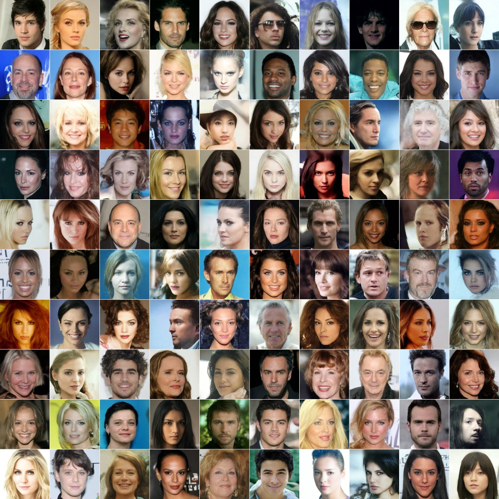
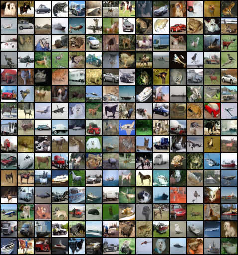
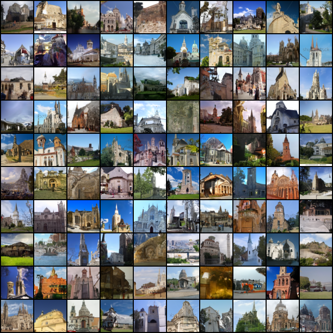
We also observe a relatively high quality of the samples too. So we get high quality and diversity! Keep in mind that quality is good, but not always as good as SOTA GANs for high-resolution images. My paper will show how to improve quality more.
GANs can only do what they are trained to do (generate full images). However, with DSM-ALS, we can do many tasks that the network was not trained to do. For example, we can do in-painting, meaning that we can start from a partially complete image and fill out the rest. This is because you can apply Langevin Sampling only on the missing parts of the image, thus fill it out! What is crazy is that we can do a lot more things too: denoising (by the design of the score matching), deblurring/super-resolution, solving inverse problems, separating two combined images, etc.
The Bad
There are two major issues: computing power and generation time.
SOTA GANs need a lot of computing power to generate high-resolution images, but it’s still more manageable than DSM-ALS. The reason is that GANs learn the mapping z->x and x->1, which makes the discriminator and generator architectures pyramidal (they decrease or increase in dimension over time). Meanwhile, with DSM-ALS, the dimension of the output must be the same as the dimension of the input (an image), and trying to reduce the dimension in the middle (U-net) does not work well in practice. Most architectures that work well only downsample once and upsample once. Because of this, we need a ton of parameters and thus, GPU RAM. 256×256 images cannot be done reliably without 8 V100 GPUs or more!!!! 🙀 So sadly, this means that only those in control of large computing resources will be able to use DSM-ALS to generate high-resolution images 😿. We have the same issue with text generation and GPT-3.
The other main issue is that generating a single image means that we need to do Langevin sampling over many steps (about 250 for 32×32 images and 2k for 256×256 images). This requires a long time. This means that this approach will never be real-time viable. Furthermore, if you want to generate lots of images, you will need large batch sizes, which means high GPU RAM. So again, you have the problem of needing a lot of expensive GPUs or TPUs to generate images at a reasonable pace (Imagine sampling 1k images with Langevin Sampling and a mini-batch of 32 😿).
As I briefly mentioned earlier, the quality of the generated samples is not always as good as SOTA GANs, but my next paper will improve on that, and the Denoising Diffusion paper already did a great job of improving quality. GANs have had many years to get to the point they are now, so it’s normal to expect a bit more time for DSM-ALS to reach its peak performance.
Another issue that I did not talk about is instability. This is because the improvements from Yang Song have fixed most of the instabilities. Having experimented with both original and improved versions, I can tell you that the original version was even more unstable than GANs! It required so much tweaking that you would go insane! 🙀 The improved version is so much better, and Yang Song gives simple recommendations for hyperparameters.
Conclusion
DSM-ALS is an incredible approach which performs better than most GANs, but comes at a high computational cost and long generation time. It will likely supersede GANs for non-real-time image generation. However, it will most likely make image generation even more out of reach for hobbyists and grad students 😿.
Watch out 🐾 for my next paper which will show how to further improve DSM-ALS 😻.
For more details, you can read both papers by Yang Song:
https://arxiv.org/abs/1907.05600
https://arxiv.org/abs/2006.09011
You can also look at the Denoising Diffusion paper by Jonathan Ho et al. which uses a similar method to generate very nice high-resolution images:
https://arxiv.org/abs/2006.11239
Samples